Plotting Piecewise Functions in Python and Matplotlib the Elegant Way, Part 2

In the previous article about piecewise functions, we talked about how to plot a piecewise function in Python using the Matplotlib library. In this article, we will discuss how a more advanced approach will allow us to adjust parameters on a piecewise plot. We will draw on the previous example of visualizing the federal tax brackets and dive into how to do it via hard-coding and soft-coding approaches.

Hard-Coding Piecewise Functions

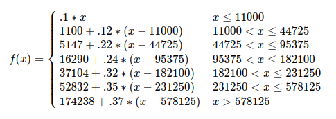
In the article where we plotted the federal tax tiers, we can see that each tax tier starts where the previous one ends. The 2023 federal tax can be represented as this function:

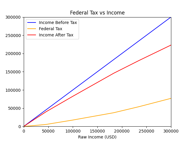
In code, we can define the piecewise function for evaluating the tax levied on the income of different tiers using a custom function wrapped inside a numpy vectorize() function.

 import matplotlib.pyplot as plt
import numpy as np


raw_income = np.arange(0, 600000, 10)

def funk(x):
    if (x >= 0) and (x < 11000):
        return 0 + 0.1 * (x - 0)
    if (x >= 11000) and (x < 44725):
        return 1100.0 + 0.12 * (x - 11000)
    if (x >= 44725) and (x < 95375):
        return 5147.0 + 0.22 * (x - 44725)
    if (x >= 95375) and (x < 182100):
        return 16290.0 + 0.24 * (x - 95375)
    if (x >= 182100) and (x < 231250):
        return 37104.0 + 0.32 * (x - 182100)
    if (x >= 231250) and (x < 578125):
        return 52832.0 + 0.35 * (x - 231250)
    if (x >= 578125) and (x < float("inf")):
        return 174238.25 + 0.37 * (x - 578125)

fed_func = np.vectorize(funk)
fed_tax = fed_func(raw_income)
post_tax = raw_income - fed_tax

plt.figure()
plt.plot(raw_income, raw_income, label='Income Before Tax', c='blue')
plt.plot(raw_income, fed_tax, label='Federal Tax', c='orange')
plt.plot(raw_income, post_tax, label='Income After Tax', c='red')
plt.legend()
plt.xlim([0, 300000])
plt.ylim([0, 300000])
plt.xlabel("Raw Income (USD)")
plt.title("Federal Tax vs Income")

Soft-Coding Piecewise Functions

The above approach may work in one-off situations. However, for every tax year, the tax brackets may change, leading to different lower bounds, upper bounds, and offsets for each tier. Therefore, there must be a better way than to define the tax tiers by hard-coding them.

From what we can see from the code above, each tax tier is in the following form, with a being the offset, a_t being the lower bound of the tax tier, b_t being the upper bound of the tax tier, and c_t being the offset of the tax tier:

This means that we can define the piecewise function more smartly via soft-coding, i.e. by specifying the boundary points and the tax rate of each tier. Actually, we would not need to supply the lower bound of each tier since each lower bound is the upper bound of the previous tier. The lower bound of the lowest tax tier is naturally going to be zero. The offset does not need to be supplied since it is the accumulated taxed amounts from all previous tiers, which lends itself well to soft-coding as well. Thus we can write a higher-order function like this:

 import matplotlib.pyplot as plt
import numpy as np
import functools


def build_function(tier_upper_bounds, rates):
    @functools.cache
    def soft_funk(x):
        tiers = []
        offset = 0
        tier_lower_bound = 0
        for i, pair in enumerate(zip(tier_upper_bounds, rates)):
            tier_upper_bound, rate = pair
            tiers.append({
                "lower_bound": tier_lower_bound,
                "upper_bound": tier_upper_bound,
                "rate": rate,
                "offset": offset
            })
            offset = offset + rate * (tier_upper_bound - tier_lower_bound)
            tier_lower_bound = tier_upper_bound
        for t in tiers:
            if (x >= t["lower_bound"]) and (x < t["upper_bound"]):
                return t["offset"] + t["rate"] * (x - t["lower_bound"])

    return np.vectorize(soft_funk)

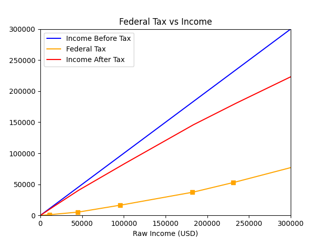
Since we are going to store the tiers’ upper bounds in arrays, this approach offers one added advantage: We can use these upper bounds to plot markers where the tax tier changes, to help the viewer spot them better. Each tier’s upper bound can be used to mark these breaking points, except for the highest tax tier which has the upper bound of infinity (i.e. the tax tier of the billionaires of this world).

We can define the tier breaking points as breaks, use the built function fed_func() to evaluate it, and add this series to the figure as a scatter plot of squares:

 raw_income = np.arange(0, 600000, 10)
tier_upper_bounds = [11000, 44725, 95375, 182100, 231250, 578125, float("inf")]
rates = [0.1, 0.12, 0.22, 0.24, 0.32, 0.35, 0.37]

fed_func = build_function(tier_upper_bounds, rates)
fed_tax = fed_func(raw_income)
breaks = tier_upper_bounds[0:-1]
post_tax = raw_income - fed_tax

plt.figure()
plt.plot(raw_income, raw_income, label='Income Before Tax', c='blue')
plt.plot(raw_income, fed_tax, label='Federal Tax', c='orange')
plt.plot(raw_income, post_tax, label='Income After Tax', c='red')
plt.scatter(breaks, fed_func(breaks), marker='s', c='orange')
plt.legend()
plt.xlim([0, 300000])
plt.ylim([0, 300000])
plt.xlabel("Raw Income (USD)")
plt.title("Federal Tax vs Income")

Unleashing More Power Out of Soft-Coding Piecewise Functions

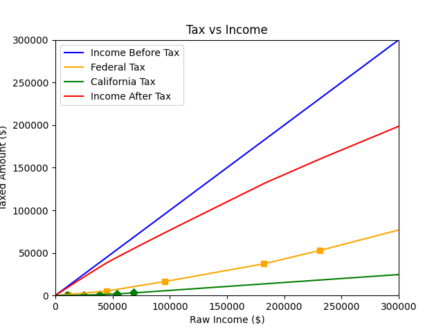
If you are not fully convinced that soft-coding saves you time, think further. As in the case of taxes that is related to income, what else is there besides the federal income tax? Well, if you live in a place besides Alaska, Florida, Nevada, New Hampshire, South Dakota, Tennessee, Texas, Washington, and Wyoming, then you would naturally need to worry about state income tax as well. To visualize the combined effects of federal and state income taxes on the same graph, would it not be great to reuse our higher-order function build_function() to help with the calculation?

And we indeed can. The state tax would not necessarily have the same tier bounds as the federal tax, and the higher-order function supports that. We just need different sets of variables for federal and state taxes in the main code to define and store them. Take California for example:

 raw_income = np.arange(0, 800000, 10)

fed_tier_upper_bounds = [11000, 44725, 95375, 182100, 231250, 578125, float("inf")]
fed_rates = [0.1, 0.12, 0.22, 0.24, 0.32, 0.35, 0.37]
fed_func = build_function(fed_tier_upper_bounds, fed_rates)
fed_tax = fed_func(raw_income)
fed_breaks = fed_tier_upper_bounds[0:-1]

cal_tier_upper_bounds = [10412, 24684, 38959, 54081, 68350, 349137, 418961, 698271, float("inf")]
cal_rates = [0.01, 0.02, 0.04, 0.06, 0.08, 0.093, 0.103, 0.113, 0.123]
cal_func = build_function(cal_tier_upper_bounds, cal_rates)
cal_tax = cal_func(raw_income)
cal_breaks = cal_tier_upper_bounds[0:-1]

post_tax = raw_income - fed_tax - cal_tax

plt.figure()
plt.plot(raw_income, raw_income, label='Income Before Tax', c='blue')
plt.plot(raw_income, fed_tax, label='Federal Tax', c='orange')
plt.scatter(fed_breaks, fed_func(fed_breaks), marker='s', c='orange')
plt.plot(raw_income, cal_tax, label='California Tax', c='green')
plt.scatter(cal_breaks, cal_func(cal_breaks), marker='D', c='green')
plt.plot(raw_income, post_tax, label='Income After Tax', c='red')
plt.legend()
plt.xlim([0, 300000])
plt.ylim([0, 300000])

plt.ylabel("Taxed Amount ($)")
plt.xlabel("Raw Income ($)")
plt.title("Tax vs Income")