Plotting Piecewise Functions in Python and Matplotlib the Elegant Way

Piecewise functions are mathematical functions that are defined by different expressions or formulas for different intervals or domains. These functions are commonly used in various fields such as mathematics, physics, and engineering to model complex systems or phenomena. In this article, we will explore how to plot piecewise functions using Python and the Numpy and Matplotlib libraries.

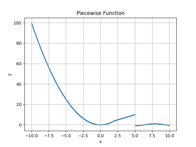
Let us take a really simple example of a piecewise function:

If you want to output to look like this:

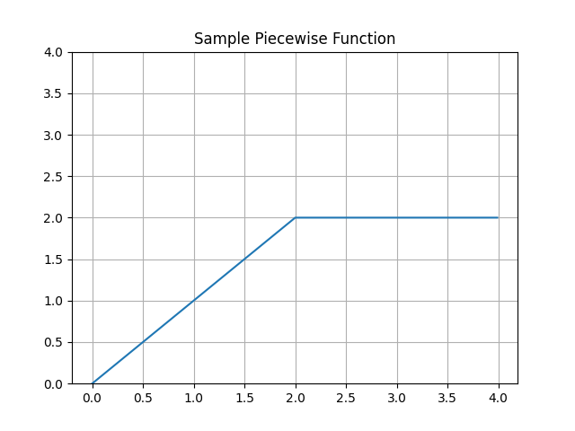
Regardless of the number of segments (i.e. pieces of functions), we would want to prepare the data on the y-axis in one series (Numpy array) rather than as several different series on the same plot. There are a couple of ways to accomplish this.

Constructing Array by vectorize() and Branching Statements

A simple way of implementing a piecewise function would be to write a Python function with conditional statements inside, and then use Numpy’s vectorize() function to apply the function to a Numpy array.

 import matplotlib.pyplot as plt
import numpy as np

def p_funk(x):
    if x <= 2:
        return x
    else:
        return 2

x_series = np.arange(0, 4, .01)
y_series = np.vectorize(p_funk)(x_series)

plt.figure()
plt.ylim(0, 4)
plt.grid(True, which='both')
plt.plot(x_series, y_series)
plt.title('Piecewise Function')

Constructing Array by piecewise() and Rules

The if/else statements above work fine, but if you want to write your code a little more like the mathematical definition (i.e. groups of expressions and conditions), there is another way. Numpy’s built-in piecewise() function has a more complicated syntax but will give more satisfaction to the mathematician in you.

 import matplotlib.pyplot as plt
import numpy as np

x_series = np.arange(0, 4, .01)
rules = [
    (lambda x: x, x_series <= 2),
    (lambda x: 2, x_series > 2),
]
evaluations, conditions = zip(*rules)

y_series = np.piecewise(x_series, conditions, evaluations)
plt.figure()
plt.ylim(0, 4)
plt.grid(True, which='both')
plt.plot(x_series, y_series)
plt.title('Sample Piecewise Function')

In the example above, we define an array of tuples, rules, as the definition of the piecewise function. The syntax of Numpy’s piecewise designates conditions and evaluations as separate arrays, but it is perfectly fine how we choose to define our rules like the mathematical expression for piecewise functions. We just have to transform the array of tuples to an array of conditions and an array of conditions.

Continuous vs Discontinuous Piecewise Functions

In the two plot examples above, the piecewise functions are continuous, meaning that each segment would start at the point where the previous segment ends. However, there are cases where mathematically, you would not want that. For example:

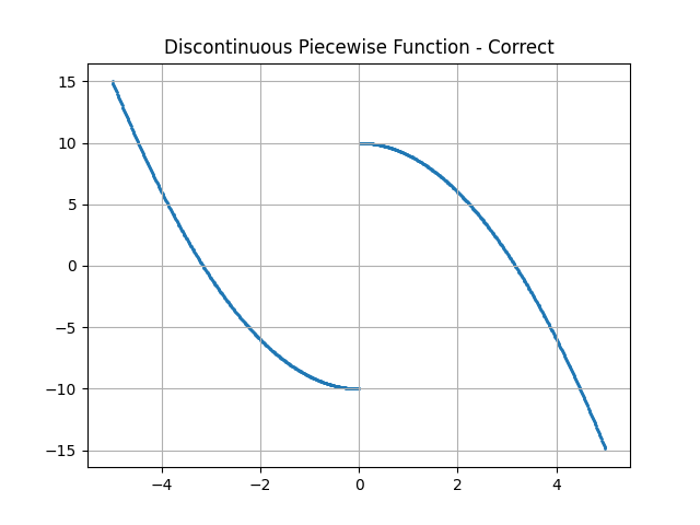
Here the two segments do not intersect at x=0, since the function is undefined at 0. Even if the function is defined at 0, the two segments still do not intersect, as the first segment evaluates to -10 and the second segment evaluates to 10 at x=0.

In this case, if we use the matplotlib.pyplot.plot() command to plot the piecewise function, the segments will be connected, since the command is more utilized for plotting continuous data. We do not want that:

 import matplotlib.pyplot as plt
import numpy as np

x_series = np.arange(-5, 5, .01)
rules = [
    (lambda x: x * x - 10, x_series < 0),
    (lambda x: -x * x + 10, x_series > 0),
]
evaluations, conditions = zip(*rules)

y_series = np.piecewise(x_series, conditions, evaluations)
plt.figure()
plt.grid(True, which='both')
plt.plot(x_series, y_series)
plt.title('Pulse Function')
plt.title('Discontinuous Piecewise Function - Incorrect')

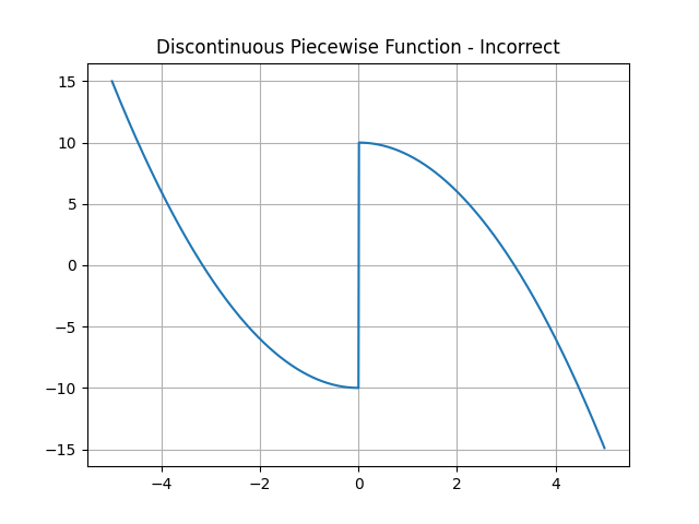
Instead, we should be using the matplotlib.pyplot.scatter() command to plot the piecewise function so that the segments will be disconnected. Although the command is usually used for plotting discrete data points, it works better than matplotlib.pyplot.plot() in this case. However, since the default scatter plot uses a somewhat large marker size, it would be wise to adjust the type of marker and its size so that the scatter plot consists of may small dots, which look like lines, except for the disconnected part.

 import matplotlib.pyplot as plt
import numpy as np

x_series = np.arange(-5, 5, .01)
rules = [
    (lambda x: x * x - 10, x_series < 0),
    (lambda x: -x * x + 10, x_series > 0),
]
evaluations, conditions = zip(*rules)

y_series = np.piecewise(x_series, conditions, evaluations)
plt.figure()
marker_style = 'o'
marker_size = 1
plt.grid(True, which='both')
plt.scatter(x_series, y_series, marker=marker_style, s=marker_size)
plt.title('Discontinuous Piecewise Function - Correct')

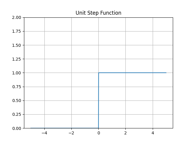
It is worth mentioning that in many cases, the matplotlib.pyplot.plot() command would work just fine. For example, in electrical engineering, certain signals are considered to be analog. In some cases, even digital signals can be drawn as continuous piecewise functions.

For example, the unit step function is usually plotted with an upshoot at x=0 connecting the two segments:

 import matplotlib.pyplot as plt
import numpy as np

x_series = np.arange(-5, 5, .01)
rules = [
    (lambda x: 0, x_series <= 0),
    (lambda x: 1, x_series > 0),
]
evaluations, conditions = zip(*rules)

y_series = np.piecewise(x_series, conditions, evaluations)
plt.figure()
plt.ylim(0, 2)
plt.grid(True, which='both')
plt.plot(x_series, y_series)
plt.title('Unit Step Function')

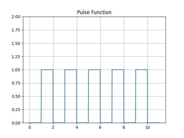
Similarly, a pulse function can be plotted using continuous connections between segments:

 import matplotlib.pyplot as plt
import numpy as np

x_series = np.arange(0, 11, .01)
rules = [
    (lambda x: 0, (x_series % 2 >= 0) & (x_series % 2 < 1)),
    (lambda x: 1, (x_series % 2 >= 1) & (x_series % 2 < 2)),
]
evaluations, conditions = zip(*rules)

y_series = np.piecewise(x_series, conditions, evaluations)
plt.figure()
plt.ylim(0, 2)
plt.grid(True, which='both')
plt.plot(x_series, y_series)
plt.title('Pulse Function')